Overview
The CamelRatiosIndex package implements the multivariate-weighted indexing method proposed by Ayimah et al. (2023a, 2023b) for bank performance assessment using the CAMEL framework. The package provides:
-
camel_index(): Computes composite year-on-year indices from CAMEL ratio data -
plot_camel_index(): Visualizes percentage differences across banks using ggplot2 - Built-in data: Example datasets from Ghanaian commercial banks (2015-2022)
This composite index is intended to offer regulators and policymakers a standardised, objective for monitoring bank performance over time and across institutions. Its ability to benchmark banks against a common base year enhances early-warning capabilities, enabling supervisory authorities to identify emerging weaknesses individual banks as well as systemic vulnerabilities within the industry.
The CAMEL Framework
CAMEL is an internationally recognized framework for evaluating bank performance, comprising five dimensions:
| Dimension | Ratio | Direction |
|---|---|---|
| Capital Adequacy | Ca | Higher = better |
| Asset Quality | Aq | Higher = worse (inverted) |
| Management Efficiency | Me | Higher = worse (inverted) |
| Earnings | Eq | Higher = better |
| Liquidity | Lm | Higher = worse (inverted) |
Installation
# Install from GitHub (development version)
# install.packages("remotes")
remotes::install_github("YOUR-USERNAME/CamelRatiosIndex")
Quick Start
Computing the CAMEL Index
library(CamelRatiosIndex)

# Load built-in example data
data("camel_2015")
data("camel_2022")

# Compute the index
result <- camel_index(camel_2015, camel_2022)
#> ℹ Using 3 factors (Kaiser criterion suggests 2 for base year).

# View the main output
result$index_table
#> # A tibble: 21 × 3
#>    bank      I_mw      PD
#>    <chr>    <dbl>   <dbl>
#>  1 Absa    116.    16.1
#>  2 AB      327.   227.
#>  3 ADB     154.    54.1
#>  4 BA       99.6   -0.420
#>  5 CB        3.72 -96.3
#>  6 Ecobank 549.   449.
#>  7 FBN     171.    70.9
#>  8 FB      151.    50.6
#>  9 FAB     204.   104.
#> 10 FNB     144.    43.7
#> # ℹ 11 more rows
Accessing Detailed Results
# Laspeyres-type indices (base year weights)
result$mw_lasp
#>  [1]  1.17068455  3.24528378  1.52780746  0.98655880  0.01257239  6.02659502
#>  [7]  1.65444746  1.54951394  2.03302237  1.49816252  2.98825411  1.28723657
#> [13]  1.13849623 -1.97551778  0.82971916  0.84601356  0.94124611  1.70736177
#> [19]  1.43859304  0.28238957  1.40351131

# Paasche-type indices (current year weights)
result$mw_pash
#>  [1]  1.15082501  3.30155142  1.55371945  1.00501635  0.06177212  4.94882308
#>  [7]  1.76427243  1.46318577  2.05241470  1.37566218  2.51395785  1.28567395
#> [13]  1.14279086 -1.80089258  0.87655232  0.79703627  0.89022374  1.65663138
#> [19]  1.43712269  0.17659450  1.42483169

# Communality weights from base year factor analysis
result$weights_base
#>        X1        X2        X3        X4        X5
#> 0.7903609 0.7050024 0.8849089 0.8942996 0.8265737

# Eigenvalues
result$eigenvalues_base
#> [1] 2.1638843 1.2551681 0.9655781 0.3240539 0.2913156
Visualizing Results
# Basic plot
plot_camel_index(result)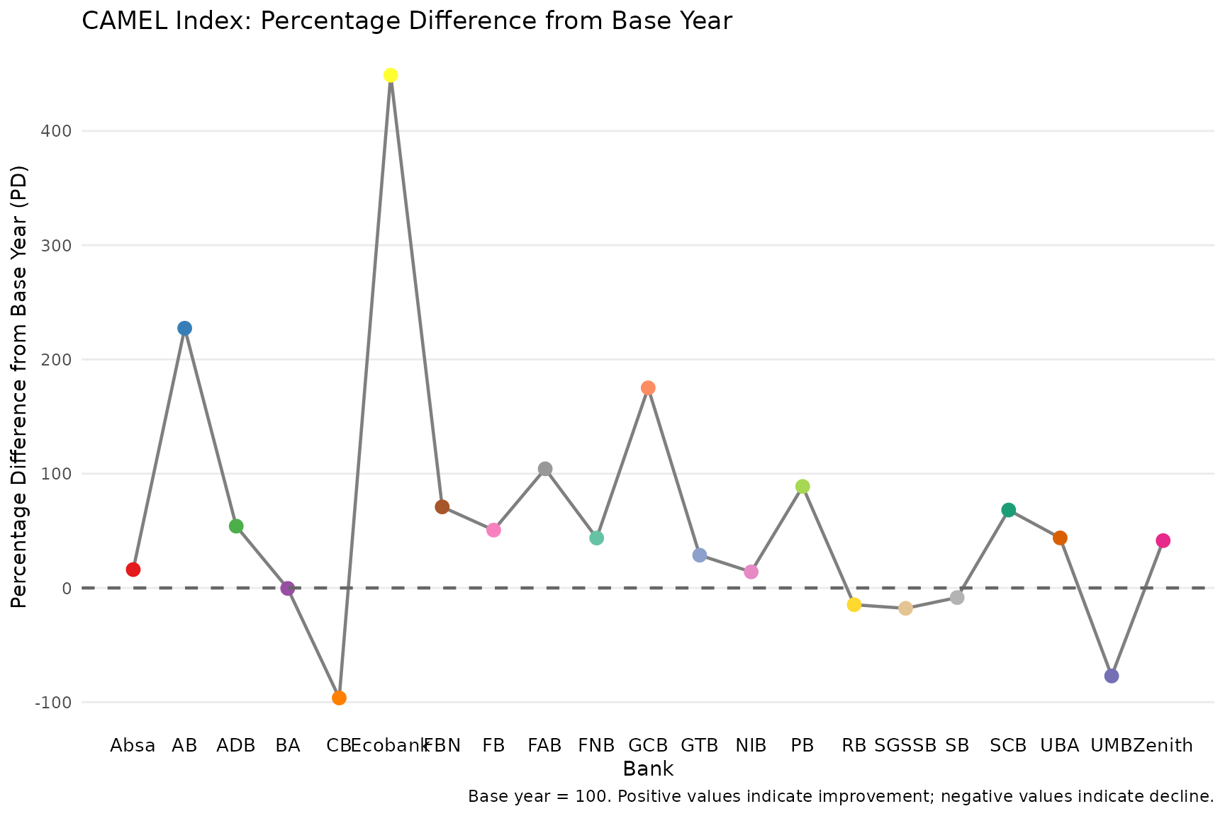
# Highlight specific banks
plot_camel_index(result, highlight_banks = c("Absa", "Ecobank", "GCB"))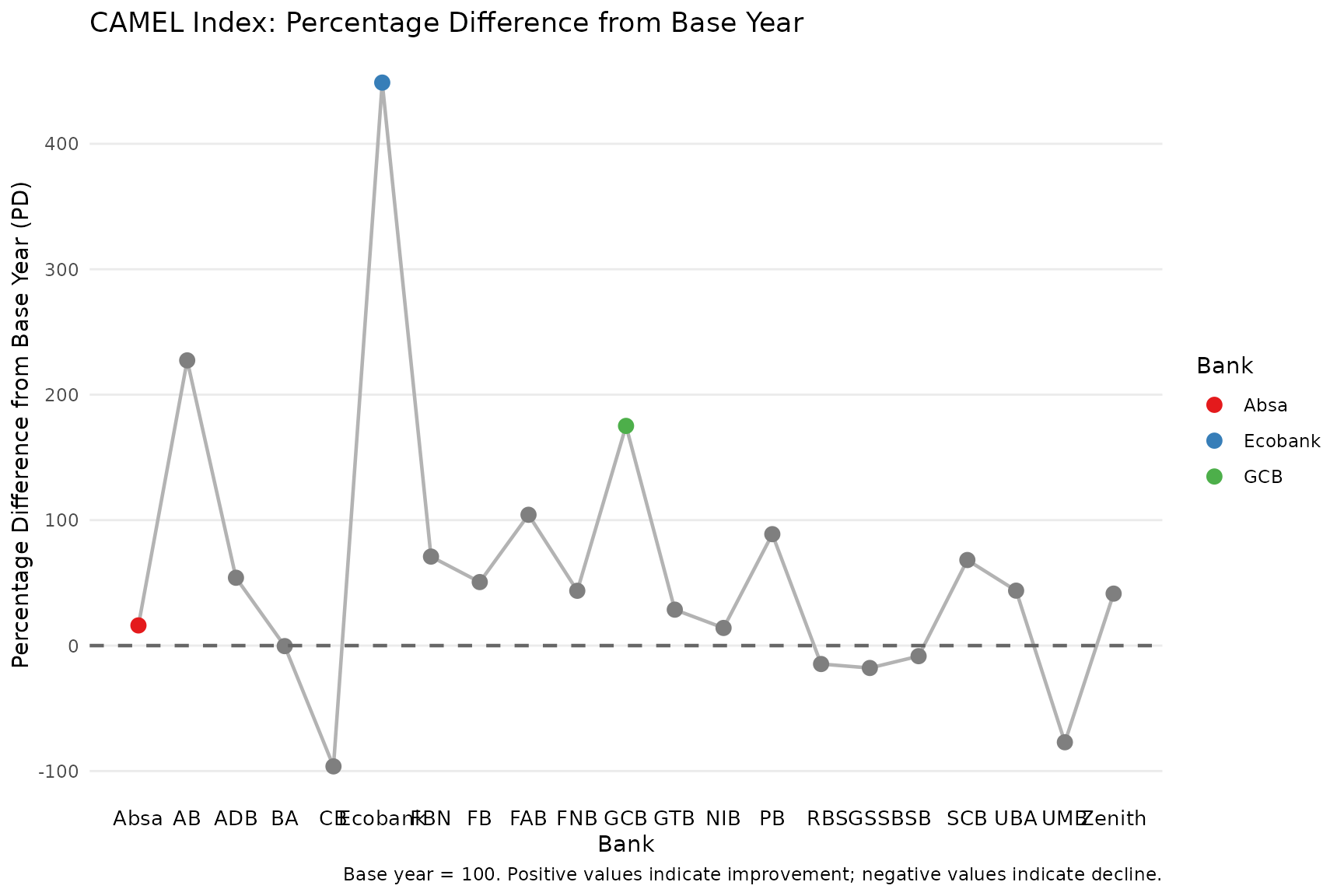
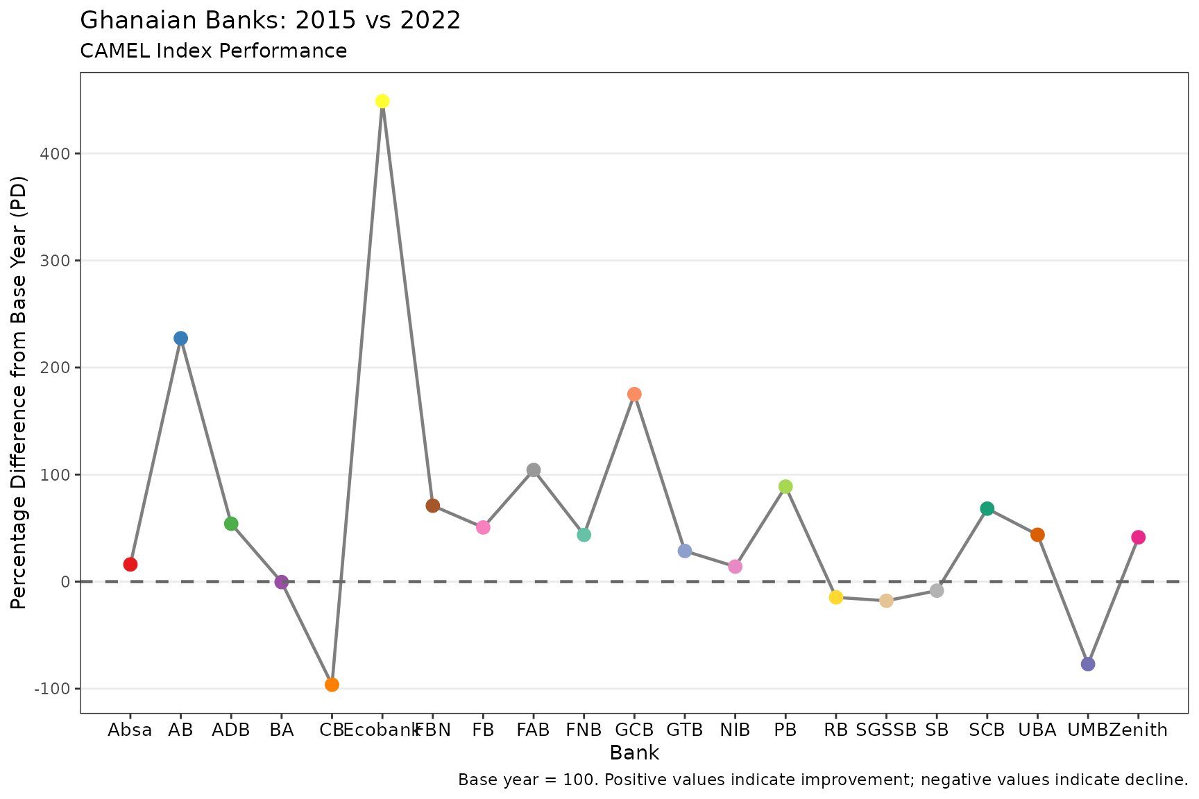
# Custom styling
plot_camel_index(
  result,
  title = "Ghanaian Banks: 2015 vs 2022",
  subtitle = "CAMEL Index Performance",
  theme_fn = ggplot2::theme_bw
)
Data Format
Data Frame Input
When using data frames, the first column must be the bank identifier, followed by the five CAMEL ratios:
# Example structure
head(camel_2015)
#> # A tibble: 6 × 6
#>   Bank      Ca1   Aq1    Me1    Eq1   Lm1
#>   <chr>   <dbl> <dbl>  <dbl>  <dbl> <dbl>
#> 1 Absa    0.178 0.187 0.04   0.087  0.714
#> 2 AB      0.059 0.084 0.0432 0.011  0.783
#> 3 ADB     0.141 0.339 0.0669 0.024  0.965
#> 4 BA      0.229 0.101 0.0353 0.0219 0.964
#> 5 CB      0.214 0.055 0.024  0.049  1.23
#> 6 Ecobank 0.171 0.180 0.451  0.055  0.699
Matrix Input
For matrices, supply bank names separately:
base_mat <- as.matrix(camel_2015[, -1])
curr_mat <- as.matrix(camel_2022[, -1])
banks <- camel_2015$Bank

result2 <- camel_index(base_mat, curr_mat, bank_names = banks)
#> ℹ Using 3 factors (Kaiser criterion suggests 2 for base year).
Understanding the Output
The camel_index() function returns a rich object with
multiple components:
# Print overview
print(result)
#>
#> ── CAMEL Index Results ─────────────────────────────────────────────────────────
#> Base year factor analysis: 2 eigenvalue(s) > 1
#> Current year factor analysis: 2 eigenvalue(s) > 1
#> Factors extracted: 3
#>
#> ── Index Table ──
#>
#> # A tibble: 21 × 3
#>    bank      I_mw      PD
#>    <chr>    <dbl>   <dbl>
#>  1 Absa    116.    16.1
#>  2 AB      327.   227.
#>  3 ADB     154.    54.1
#>  4 BA       99.6   -0.420
#>  5 CB        3.72 -96.3
#>  6 Ecobank 549.   449.
#>  7 FBN     171.    70.9
#>  8 FB      151.    50.6
#>  9 FAB     204.   104.
#> 10 FNB     144.    43.7
#> # ℹ 11 more rows
#> ── Communality Weights (Base Year) ──
#> # A tibble: 5 × 2
#>   ratio  weight
#>   <chr>   <dbl>
#> 1 Ratio1  0.790
#> 2 Ratio2  0.705
#> 3 Ratio3  0.885
#> 4 Ratio4  0.894
#> 5 Ratio5  0.827
#> ── Summary Statistics ──
#> Mean I_mw: 160.05
#> Mean PD: 60.05%
#> Best performing bank: Ecobank (PD = 448.77%)
#> Worst performing bank: CB (PD = -96.28%)

# Detailed summary
summary(result)
#>
#> ── CAMEL Index Summary ─────────────────────────────────────────────────────────
#>
#> ── Eigenvalues (Base Year) ──
#>
#> # A tibble: 5 × 3
#>   component eigenvalue variance_pct
#>   <chr>          <dbl>        <dbl>
#> 1 PC1            2.16         43.3
#> 2 PC2            1.26         25.1
#> 3 PC3            0.966        19.3
#> 4 PC4            0.324         6.48
#> 5 PC5            0.291         5.83
#> ── Eigenvalues (Current Year) ──
#> # A tibble: 5 × 3
#>   component eigenvalue variance_pct
#>   <chr>          <dbl>        <dbl>
#> 1 PC1            2.06         41.1
#> 2 PC2            1.43         28.7
#> 3 PC3            0.788        15.8
#> 4 PC4            0.524        10.5
#> 5 PC5            0.199         3.97
#> ── Factor Loadings (Base Year) ──
#> # A tibble: 5 × 4
#>   ratio   Factor1  Factor2 Factor3
#>   <chr>     <dbl>    <dbl>   <dbl>
#> 1 Ratio1  0.835    0.0532    0.302
#> 2 Ratio2  0.766    0.00678  -0.343
#> 3 Ratio3 -0.162    0.920     0.114
#> 4 Ratio4 -0.00290  0.0102    0.946
#> 5 Ratio5 -0.469   -0.762     0.160
#> ── Index Distribution ──
#> # A tibble: 7 × 3
#>   statistic   I_mw      PD
#>   <chr>      <dbl>   <dbl>
#> 1 Min         3.72 -96.3
#> 2 Q1         99.6   -0.420
#> 3 Median    144.    43.7
#> 4 Mean      160.    60.1
#> 5 Q3        171.    70.9
#> 6 Max       549.   449.
#> 7 SD        115.   115.
Key Metrics
- I_mw: Composite index (base = 100). Values > 100 indicate improvement; < 100 indicate decline.
- PD: Percentage difference from base year. Positive = improvement.
- mw_lasp: Laspeyres-type index using base year communality weights.
- mw_pash: Paasche-type index using current year communality weights.
- weights_base/current: Communality values from robust factor analysis, representing the proportion of variance explained by each CAMEL ratio.
Methodology
The index computation follows these steps:
- Transform ratios: Invert Aq, Me, and Lm so that higher values always indicate better performance.
- Compute correlations: Build correlation matrices for base and current years.
- Extract eigenvalues: Determine the number of factors (eigenvalues > 1).
- Robust factor analysis: Use [robustfa::FaCov()] with OGK covariance estimation.
- Extract communalities: Use communalities as weights for each CAMEL ratio.
- Compute indices: Calculate Laspeyres and Paasche indices, then average them.
- Scale to base 100: Final composite index with percentage difference.
References
Ayimah, J. C., Mettle, F. O., Nortey, E. N., & Minkah, R. (2023a). A Robust Multivariate Weighting Technique for Computing a Measure for Inflation. African Journal of Technical Education and Management, 3(1), 1-15. Retrieved from https://ajtem.com/index.php/ajtem/article/view/53.
Ayimah, J.C. (2023b). Computing Multivariate-Weighted Consumer Price Index: An Application Manual in R. B P International. DOI: 10.9734/bpi/mono/978-81-19315-32-1. DOI:http://dx.doi.org/10.9734/bpi/mono/978-81-19315-32-1